Introduction
Have you ever wondered how life’s most basic units, cells, operate? As a programmer and cell biology enthusiast, I embarked on a journey to simulate the simplest cell using TypeScript. Cells are incredibly complex, scientists estimate that an average human cell has 100 trillion atoms. We still know very little about how all these molecules interact with each other, thus making it impossible to perform an exact simulation.
This is when I found the paper Fundamental behaviors emerge from simulations of a living minimal cell. Using kinetic parameters, they create a model of the molecules and reactions in the simplest known cell. They then run a simulation and are able to observe processes like DNA replication, metabolism and protein synthesis.
I wanted to understand what they did by reproducing it in Typescript and thus also making the simulation easily available to run in the browser without any installation. This article will focus on the well-stirred model, which models the whole cell as a single homogeneous mixture. In the paper, the well-stirred model is calibrated and verified using a more advanced “spatial” model that uses a 3D grid to also account for movement of molecules throughout the cell.
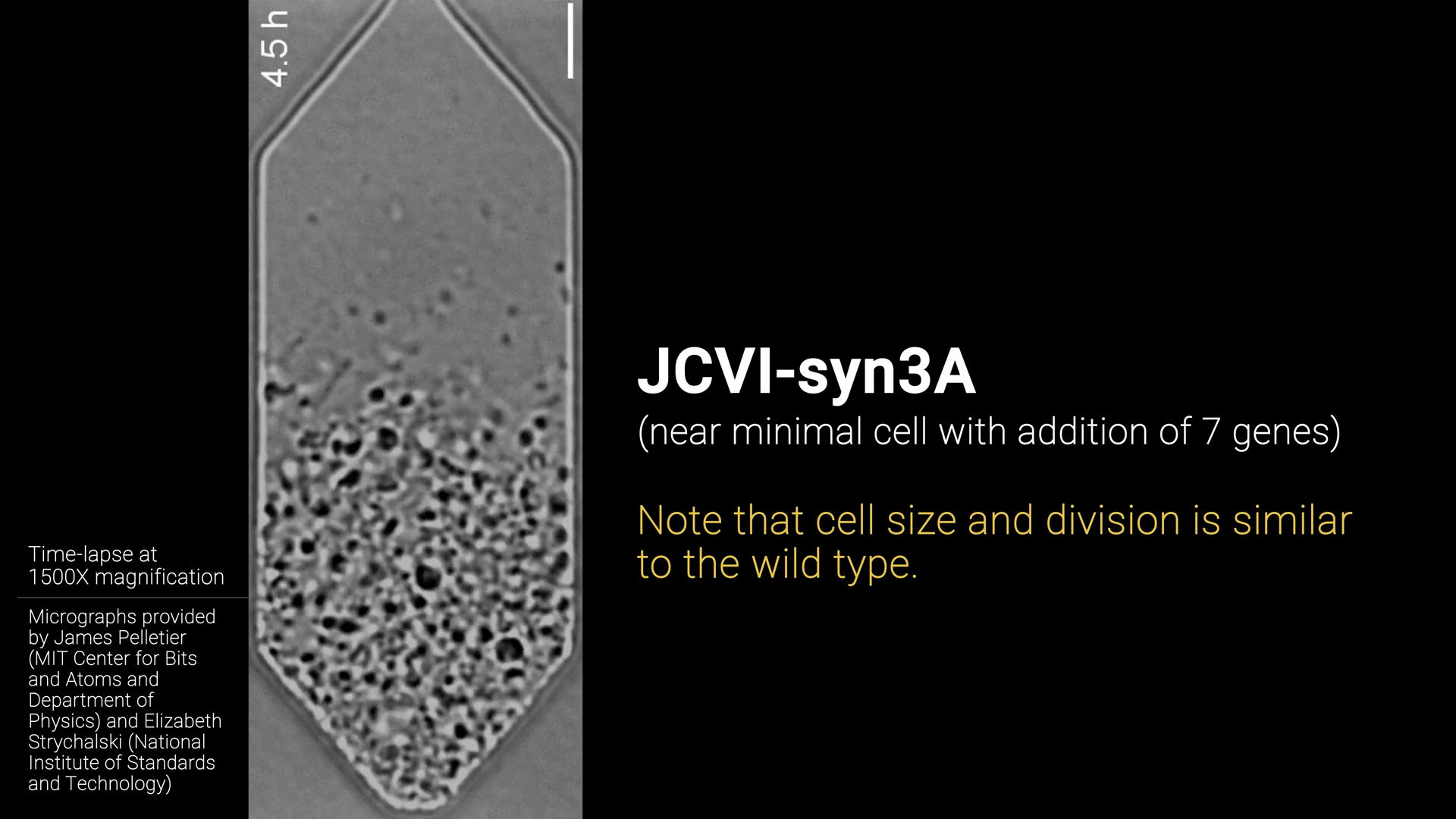
Minimal cell (JCVI-syn3A)
In order to simulate a cell we need to know as much as we can about the genes, proteins and metabolism inside the cell. Most of this is still unknown to science, especially in relatively large and complex cells like those of animals. Therefore scientists decided to create a cell with the smallest possible complixity (number of genes).
They did this by starting with a bacterial cell and removing genes until it could not survive anymore. This way they knew they had gone to far, and this gene was apparently critical for survival. Using this method, they mapped out which genes where critical and which where not. Until they finally arrived at the minimal cell JCVI-syn3A.
The result is a genetically minimal bacterial cell with “only” 493 genes. Compare that to another bacteria “E. Coli.” which has 4637 genes and you can see why they did this. Of the 493 genes only 20% is unclear in function, so scientists have enough information to start putting together a model for this cell. This is exactly what they did in Kinetic Modeling of the Genetic Information Processes in a Minimal Cell. The resulting kinetic parameters are the foundation of the simulation we will build.
Genome data
All data is publicly available in the GitHub repository from the Luthey Schulten Lab.
The entire genome is stored in the file syn3A.gb. This is a GenBank file that contains the DNA code and information about the genes and which proteins they code for. For example we can see that the gene in position 497075..498190 creates the protein Dihydrofolate synthase. Which consists of the amino acids MISV…NNKF. Where M = Methionine, I = Isoleucine, etc…
complement(497075..498190)
/gene="folC"
/locus_tag="JCVISYN3A_0823"
/product="Dihydrofolate synthase"
/protein_id="AVX54985.1"
/translation="MISVDQELFPINQRLNKEVVFDKVLDELNHPEEFLKVINVVGTN
GKGSTSFYLSKGLLKKYQKVGLFISPAFLYQNERIQINNTPISDNDLKSYLHKIDYLI
KKYQLLFFEIWTLIMILYFKDQKVDIVVCEAGIGGIKDTTSFLTNQLFSLCTSISYDH
MDILGNSIDEIIYNKINIAKPNTKLFISYDNLKYKDKINEQLINKNVELIYTDLYEDQ
IIYQQANKGLVKKVLEYLNIFQTNIFQLQPPLGRFTTIRTFPNHIIIDGAHNVDGINK
LIQSVKMLNKEFIVLYASITTKEYLKSLELLDQNFNEVYICEFNFIKSWSIDNIDHKN
KIKDWKKFLKNNTKNIIICGSLYFIPLVYNYLTNNKF"
Kinetic parameters
The kinetic parameters are stored in SBTab files, like this file which includes the reactions for the central metabolism. These files contain the initial concentrations, reactions between the metabolites and formulas and parameters used to calculate the reaction rate (speed).
For example, the initial concentration of ATP (denoted as M_atp_c) is 3.6529 millimolar (mM).
One of the reactions it appears in is M_atp_c + M_f6p_c <=> M_adp_c + M_fdp_c which converts Fructose 6-phosphate into Fructose 1,6-bisphosphate and uses up one ATP to do it.
The rate formula can be seen below:
( 0.001 / 1.0) * (( kcrg_R_PFK * ( ( ((keq_R_PFK)^(hco_R_PFK/2.)) * M_atp_c * M_f6p_c) - (((keq_R_PFK)^(-hco_R_PFK/2.)) * M_adp_c * M_fdp_c) ) )) / sqrt(kmc_R_PFK_M_atp_c * kmc_R_PFK_M_f6p_c * kmc_R_PFK_M_adp_c * kmc_R_PFK_M_fdp_c) / (( (1 + (M_atp_c/kmc_R_PFK_M_atp_c)) * (1 + (M_f6p_c/kmc_R_PFK_M_f6p_c)) ) + ( (1 + (M_adp_c/kmc_R_PFK_M_adp_c)) * (1 + (M_fdp_c/kmc_R_PFK_M_fdp_c)) ) - 1)
Each of the parameters here is also defined in the last part of the file, for example kmc_R_PFK_M_atp_c = 0.117.
Chemical Master Equation (CME)
In order to simulate the genetic systems the paper uses the chemical master equation. This method is used to simulate stochastic (random) systems. The following functions are simulated in the CME:
- DNA transcription to mRNA
- mRNA translation to proteins
- mRNA degradation
- DNA replication
- tRNA charging
The name “chemical master equation” sounds very complicated, but what it boils down to is actually a very simple algorithm, called the Gillespie algorithm. At every time t, we calculate the “propensity” for each reaction, which is the rate multiplied by the concentration of the reactants. We choose a random timestep to advance the simulation by, based on the total propensity. The higher the total propensity, the smaller the average timestep will be.
Δt = (1 / totalPropensity) * ln(1 / randomNumber)
We then pick a random reaction, the higher the propensity the higher the chance to be picked. This reaction is then “executed”, and the concentrations are adjusted to reflect this. And thats it, we just repeat this until we reached our target time and then return the resulting concentrations.
So what happens in practice is that we are constantly picking random genes to be translated to mRNA and random mRNA strings to be translated to proteins. This results in variation between different cells. Some cells grow quicker, or start DNA replication sooner. When running the program multiple times, you get a different result each time, just like you would in the real world.
Ordinary Differential Equation (ODE)
The metabolic reactions are calculated deterministically (not random) using an ordinary differential equation (ODE). The different systems that are included are:
- Central metabolism
- Lipid metabolism
- Nucleotide metabolism
- Amino acid metabolism
- Cofactor metabolism
- Transport reactions
Differential equations are very common in computer software. For example when creating a game, one often simulates movement by constantly increasing the position with the velocity multiplied by Δt. In this case the velocity is the derivative of the position.
In our biological simulation, the concentrations are increased by the reaction rates multiplied by Δt. For each metabolite we count up the reactions that consume it, and the reactions that produce it. This produces a very large derivative function, which is very “stiff”. Stiff means that the function is very unstable and quickly goes to infinity when not integrated carefully.
To solve this differential equation we need to use a specialised integration method called LSODA. This algorithm constantly checks the error and adjusts the timestep size to keep the integration stable. LSODA was originally written in 1983 using the programming language Fortran. But thankfully there is the project libsoda that has a C version of the code.
Using the tool Emscripten its possible to compile this code to Web Assembly (WASM), so we can run it in the browser.
This has the added advantage that its really fast, because Web Assembly runs directly on the CPU which makes it much faster than JavaScript.
Communication between CME and ODE
We now have two separate systems, the CME for genetic processes and the ODE for metabolism. To combine these we need to have some form of communication between them.
The base of the simulation is the CME, this is initialised with the initial concentrations. After every second of simulation, the CME particles are converted to ODE concentrations and written to the ODE. The ODE is then integrated for 1 second and the resulting concentrations are converted back to particles and written to the CME. This is repeated until the simulation end time is reached.
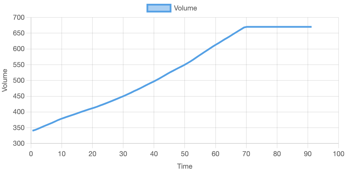
Results
Below you can see the results from one of the simulations. After comparing them to the results in the paper, they seem to be similar and thus validate the correctness of the simulation. Over multiple runs, the volume reaches the maximum of 6.7e-17 L around 60 - 70 minutes.
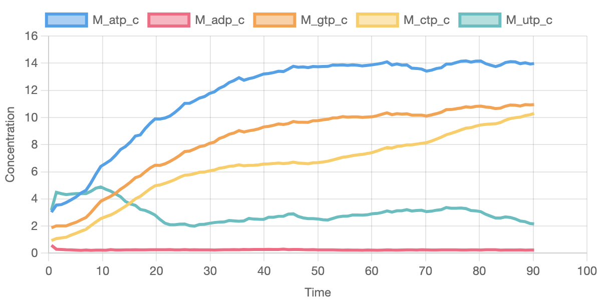
The graph below shows some of the pools of available metabolites.
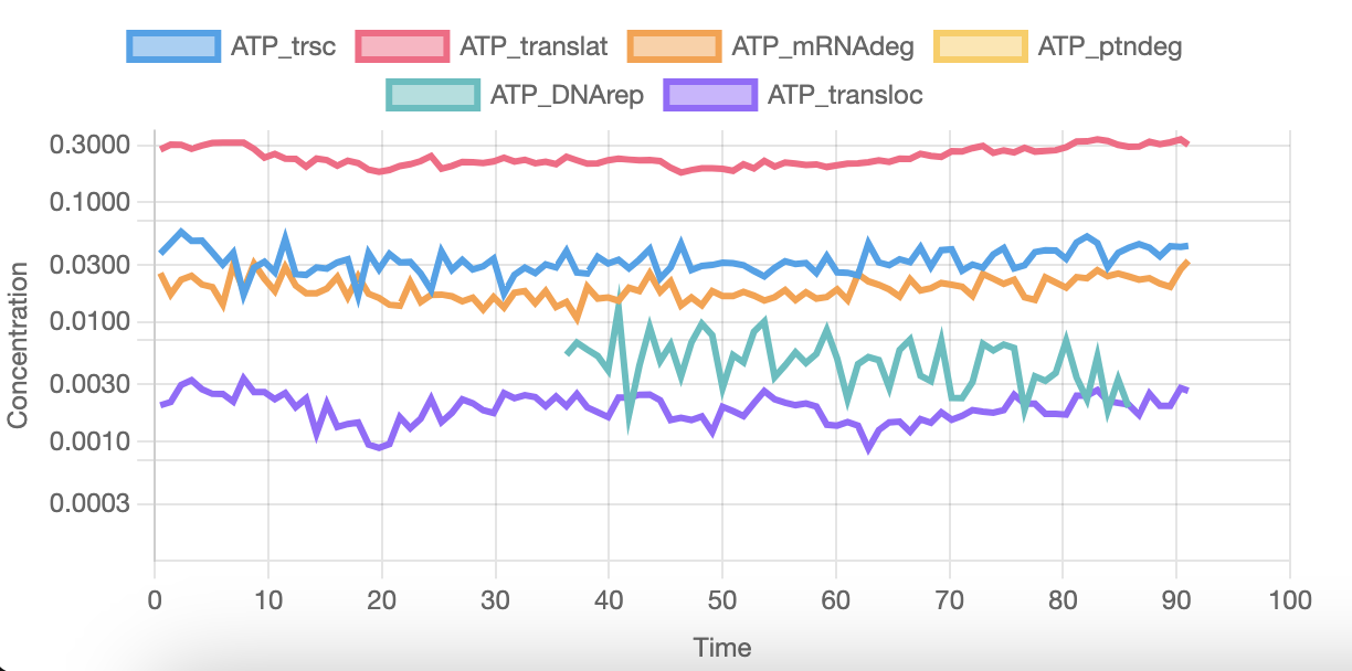
And this last graph shows the ATP usage on several activities. As you can see, DNA replication starts at around 35 minutes and completes 85 minutes into the simulation. This varies a lot across runs, and can start from as early as 5 minutes into the simulation. Sometimes it even replicates the complete genome twice.
With some optimisations the performance is also quite good, simulating a full cycle in around 20 minutes on a 5 year old MacBook. This happens in the browser and on a single thread, so with web workers it would be able to run multiple simulations in parallel.
Future
The simulation does not include any cell cycle mechanics at the moment. So cell division is done in the paper using a rule based approach. In my opinion this is an obvious next research area to explore in the future. Another goal is to scale this up to more complicated cells like human cells, which would be very interesting to easily study the effects of drugs.
The next frontier is a full molecular dynamics simulation of an entire cell. In this kind of simulation, you simulate each atom (or small groups of atoms) individually, which is much closer to reality. This is being worked on in some initial research, for example the paper Molecular dynamics simulation of an entire cell. At the moment scientists are still missing a lot of data and software capabilities, so this will probably take a long time before becoming a reality.
Demo and code
You can run the simulation yourself on my website.
The complete source code for this project is publicly available on my GitHub.
Discuss on Hacker News